My first Multi-GPU kernel: Writing All-to-all for AMD MI300X
Last month, I participated in the AMD Distributed Challenge, hosted by GPU MODE. This was very exciting for me as it was the first time I learned how to write a multi-GPU kernel! Although I had a brief understanding of how DDP and FSDP worked under the hood via collective primitives like all-reduce and reduce-scatter, I didn’t know it was possible to perform remote memory access directly inside a kernel! It opens up a lot of opportunities for multi-GPU optimizations, especially overlapping compute with inter-GPU communications.
This blog post is structured as my worklog on the 1st problem - All-to-All kernel. You can see the full problem description, including the reference kernel, at gpu-mode/reference-kernels. I also released all of my messy solutions developed during the competition without any further touch-ups (mainly because I was too lazy to do so) at gau-nernst/gpu-mode-kernels.
Problem Description
Single-GPU MoE
Before describing the problem, let’s briefly review the architecture of Mixture-of-Expert (MoE) models. An MoE layer typically consists of multiple experts, only some of which are active for each token at runtime. There is a small router deciding which experts are selected for a particular token. DeepSeek-V3 activates 8 out of 256 total experts for each token.
Implementation-wise, imagine we are processing M tokens, then we have the following tensors:
- Input tokens, shape
(M, dim) - Top-k indices showing which experts are selected for each token, shape
(M, topk) - Top-k weights for weighted average after each selected experts process their share of inputs, shape
(M, topk)
When M is somewhat large, the input data is not in an ideal layout - tokens assigned to a particular expert might be scattered all over the place in the input tokens tensor, making efficient data loading hard. A common solution to this problem is grouping tokens belonging to the same expert together. For the single-GPU case, vLLM calls this moe_align_block_size() (which was taken from SGLang?).
- I don’t know the historical context of this naming, but it feels kinda weird to focus the name on the “align block size” aspect (if I recall correctly, it pads the expert boundaries so that inputs for each expert are multiples of
BLOCK_M). I think this is not necessary anyway.
After grouping the tokens, we can perform Grouped GEMM, which is a fancy way to say doing multiple matmuls in one kernel. This is important because we don’t want to launch 256 GEMM kernels separately, each of which may only perform a small GEMM. The results from all experts can then be sent back to their original positions, scaled by their topk_weights, and summed up across topk tokens.
- When we transform the input tokens to grouped GEMM layout using a particular mapping, it’s a gather operation. When we restore the original layout using the same mapping, it’s a scatter-reduce operation. We have a “reduce” because each original token is indexed
topktimes, hence there will betopktokens from grouped GEMM outputs going back to the same location.

Tokens rearrangement in single-GPU MoE. Gather groups tokens assigned to the same expert together. Grouped GEMM performs MLP. Scatter-Reduce aggregates the results back to the original token positions.
Multi-GPU MoE
In the multi-GPU case with Expert-Parallelism (EP), it’s not very different from the algorithm described above, though they have new names. dispatch sends tokens to their respective experts, which are now sharded across GPUs. combine sends grouped GEMM outputs back to their original GPU and positions.
EP is usually enabled together with Data-Parallelism (DP). Each GPU holds a disjoint set of tokens i.e. input data is sharded. dispatch sends data from all GPUs to “all” other GPUs, and similarly for combine, hence the name all-to-all.

Tokens rearrangement in multi-GPU MoE. This diagram is exactly the same as the single-GPU one. The only difference is the extra space signifying a cross-GPU boundary.
The problem is then to implement dispatch() and combine() kernels. Sounds simple enough!
Optimized PyTorch-only solution
The reference kernel is quite slow because there are lots of Python loops. Eliminating them was my first goal.
I briefly spent some time studying MoE kernels before, thus I know that sorting is one way to group tokens belonging to the same expert together. A single-GPU version can be implemented as follows.
def moe(inputs: Tensor, moe_weights: Tensor, topk_indices: Tensor, topk_weights: Tensor):
    # inputs:       (M, dim)
    # moe_weights:  (num_experts, dim, dim)
    # topk_indices: (M, topk)
    # topk_weights  (M, topk)

    M, dim = inputs.shape
    num_experts, _, _ = moe_weights.shape
    _, topk = topk_indices.shape

    # notice we flatten the indices tensor.
    sort_indices = topk_indices.view(-1).argsort()  # (M * topk,)

    # get the token position in `inputs`, then perform gather.
    sorted_pos = sort_indices // topk
    grouped_gemm_inputs = inputs[sorted_pos]  # (M * topk, dim)

    # count number of tokens per expert to determine expert boundaries.
    # your actual grouped GEMM kernel may require a different layout/metadata.
    experts_count = topk_indices.view(-1).bincount(minlength=num_experts)
    cu_experts_count = experts_count.cumsum(dim=0).to(torch.int32)

    # perform grouped GEMM.
    # in an actual MoE, each expert is an MLP, not just a matmul.
    grouped_gemm_outputs = torch._grouped_mm(
        grouped_gemm_inputs,
        moe_weights.transpose(-1, -2),
        cu_experts_count,
    )

    # apply topk weights. this should be fused with scatter-reduce instead.
    grouped_gemm_outputs *= topk_weights.view(-1)[sort_indices].view(-1, 1)

    # perform scatter-reduce to aggregate the tokens to their original positions.
    outputs = inputs.new_zeros(M, dim)
    sorted_pos_expanded = sorted_pos.view(-1, 1).expand(-1, dim)  # scatter_add_() does not broadcast
    outputs.scatter_add_(dim=0, index=sorted_pos_expanded, src=grouped_gemm_outputs)

    return outputs
We can use this idea to improve the reference kernel. In dispatch(), each GPU can sort and do an expert count on its own local tokens. Then, all GPUs collectively perform a non-uniform all-to-all (dist.all_to_all_single() in PyTorch) to obtain tokens assigned to their local experts. This is, in fact, the same as the reference kernel, with tokens sort replacing Python for loops in the tokens rearrangement phase.
Post-all2all, tokens are in their assigned GPUs, but they are not fully sorted according to their local expert assignment. This is not a big issue: we can do another sort to get the correct grouped GEMM input layout.
- The tokens are partially sorted within each source GPU group, but we can’t exploit this fact without a custom kernel.

PyTorch-only implementation of dispatch.
Since this problem focuses on the dispatch() and combine() kernels, grouped GEMM is simulated with a simple pointwise multiplication.
For combine(), as discussed in the Problem Description section, it’s the inverse of dispatch(). We perform gather twice in dispatch(), once in the original GPU, and once in the grouped GEMM GPU. Thus, in combine(), we also do scatter twice in the reverse order. Looking at the diagram above, you can invert the arrow directions to obtain the flow of combine().
This was my submission_v2.py. On the leaderboard, this version achieves 1,311μs, compared to the reference kernel’s 93,540μs. The speedup didn’t really mean much, as the reference was intentionally poorly implemented. At this point, I thought there wasn’t much headroom left for a PyTorch-only implementation. Hence, I started looking into HIP implementations.
A brief introduction to multi-GPU programming
Peer-to-Peer (P2P)
Before talking about custom HIP kernels, let’s discuss Peer-to-Peer (P2P) and Symmetric memory, the fundamental building blocks of multi-GPU communications. P2P memory access can be broadly understood as the ability for devices to read from and write to memory of other devices. This is very powerful as we can write custom kernels that perform remote memory access directly, in any patterns we want, without launching separate communication kernels or issuing Direct Memory Access (DMA) commands. Ironically, I read CUDA C++ documentation to understand P2P usage on MI300X, though it also means that AMD’s strategy of mirroring CUDA API in HIP has some benefits.
To use P2P, it’s quite simple.
constexpr int WORLD_SIZE = 8;

int main() {
  int rank = ...; // assigned GPU rank
  CUDA_CHECK(cudaSetDevice(rank)); // switch to this particular GPU's CUDA context

  // on each GPU, allocate memory and get its memory handles
  char *ptr;
  int size = 1 << 30; // 1 GiB
  CUDA_CHECK(cudaMalloc(&ptr, size));

  cudaIpcMemHandle_t h;
  CUDA_CHECK(cudaIpcGetMemHandle(&h, ptr));

  // exchange memhandles somehow
  // since we have PyTorch, we can just call all-gather
  cudaIpcMemHandle_t all_handles[WORLD_SIZE];

  // "open" memory handles i.e. map remote memory addresses
  // in the current CUDA context's address space.
  char *all_ptrs[WORLD_SIZE];
  for (int i = 0; i < WORLD_SIZE; i++) {
    if (i == rank)
      all_ptrs[i] = ptr;
    else
      CUDA_CHECK(cudaIpcOpenMemHandle(reinterpret_cast<void **>(all_ptrs + i),
                                      all_handles[i],
                                      cudaIpcMemLazyEnablePeerAccess));
  }

  // then you can pass pointers of remote memory to kernels
  // and deference them as usual
}
PyTorch doesn’t expose these functionalities directly, so I had to write small wrappers for the CUDA/HIP functions above (though PyTorch does use them internally for things like sending CUDA tensors across processes in torch.multiprocessing). There are extra hoops you can jump through, like cudaDeviceCanAccessPeer() and cudaDeviceEnablePeerAccess(), but they are not necessary if your setup already supports P2P (and if it doesn’t, you will get an error anyway).
P2P can be backed by different transport layers, such as PCIe, NVLink (NVIDIA), and xGMI (AMD). On NVIDIA GPUs, you can use nvidia-smi topo -p2p rw and nvidia-smi topo -m to check for P2P support and the underlying interconnect.
nvidia-smi topo -p2p rw
        GPU0    GPU1    GPU2    GPU3
 GPU0   X       CNS     CNS     OK
 GPU1   CNS     X       OK      CNS
 GPU2   CNS     OK      X       CNS
 GPU3   OK      CNS     CNS     X

nvidia-smi topo -m
        GPU0    GPU1    GPU2    GPU3
GPU0     X      PHB     PHB     NV4
GPU1    PHB      X      NV4     PHB
GPU2    PHB     NV4      X      PHB
GPU3    NV4     PHB     PHB      X
For AMD GPUs, following Iris, I used fine-grained memory for buffers used for remote access. I’m not particularly sure what it is doing, and whether it is necessary, but following Iris is probably not a bad idea.
Symmetric memory & Symmetric heap
Based on my understanding, symmetric memory can be seen as memory of the same size allocated on each GPU, and peer-accessible to all other GPUs. OpenSHMEM’s section on Symmetric Data Objects gives a more formal definition. In other words, any memory allocations that have their IPC memory handles shared across all GPU processes can be considered symmetric.
If we just do the allocation once, and slice data from it as needed, it becomes a symmetric heap!
class P2PState:
    def __init__(self, rank: int, world_size: int, size: int = 1 << 30) -> None:
        # allocate a large chunk of memory. same size across ranks
        self.heap = torch.empty(size, dtype=torch.uint8, device="cuda")
        self.ptr = 0
        self.size = size

        # exchange IPC mem handles -> this becomes a symmetric heap
        ...

    def malloc_symmetric(self, shape: tuple[int, ...], dtype: torch.dtype, alignment: int = 128) -> Tensor:
        start = triton.cdiv(self.ptr, alignment) * alignment
        end = start + math.prod(shape) * dtype.itemsize
        assert end <= self.size
        out = self.heap[start:end].view(dtype).view(shape)
        self.ptr = end
        return out
The only caveat to take note of is that each allocation must be identical across all ranks. You can’t allocate (4, 128) of FP32 on symmetric heap on rank 1, but do (7, 128) of BF16 on rank 2 at the same. This restriction naturally comes from how we index into remote allocations as I will explain below.
When we slice symmetric memory from a symmetric heap, we don’t have the exact memory address of remote allocations. We only have the heap bases of all other GPUs when we do IPC memory handles exchange. Using the translate trick (I borrow the term from Iris), we can then find the exact address of a symmetric object in any other ranks.
template <typename T>
__device__ __host__
T *translate(T *ptr, int64_t src_base, int64_t dst_base) {
  static_assert(sizeof(ptr) == sizeof(int64_t));
  const int64_t offset = reinterpret_cast<int64_t>(ptr) - src_base;
  return reinterpret_cast<T *>(dst_base + offset);
}
This only works if the object’s offset from the heap base is the same across all GPUs. We maintain this invariance by ensuring that all symmetric allocations have the same size across ranks.
The main advantage of using a symmetric heap is that it’s more convenient: you only need to carry one set of heap bases around for all symmetric allocations, instead of one set of addresses for each allocation.
Acquire-Release semantics
When I studied pplx-kernels and triton-distributed, I came across these foreign words: acquire and release. I had no idea what they meant! Luckily, I found this amazing blogpost from Dave Kilian explaining the concepts in clear detail.
In a typical communication kernel, you have a producer and a consumer. The producer writes some data, and the consumer reads that data. The tricky part is synchronization: how does the consumer know when the data has arrived, and when it is safe to read it? We can use a signal flag for this.
- The flag is initialized to
0, meaning the data has not arrived. - Once the producer has finished writing the data it wants to send, it can set this flag to
1. - From the consumer side, it does a spin-lock: continuously check if the flag is
1. If it is, then the consumer can proceed to read the transferred data safely.
However, there is no guarantee of memory ordering between two memory instructions without additional constraints. When we write A and B sequentially, B may arrive before A. Similarly, when we read C and D sequentially, D may be fetched before C. This is not a limitation of C/C++, but a built-in contract between the Instruction Set Architecture (ISA), down to the assembly level, and the programmer.
This is highly problematic for us. It means that when the consumer sees flag = 1, it doesn’t mean the data has arrived. The consumer may also prefetch the data before seeing flag = 1. This is why we need memory semantics. In our particular case, what we need is Acquire-Release semantics, which are explained beautifully in Dave Kilian’s blog post above.
In summary, what you need to know is:
- As a producer, once you have finished writing the data, you set a flag with release semantics. This ensures all memory writes prior to the flag store have finished before the flag is set.
- As a consumer, you check for the flag with acquire semantics before reading the data. This ensures no data reads after the flag read are executed before the flag is observed to be set.
def producer(data, flag):
    # write some data
    data[0] = 1
    data[1] = 2

    # signal data has arrived, using release semantics
    store_release(flag, 1)

def consumer(data, flag):
    # spinlock using acquire semantic
    while load_acquire(flag) == 0:
        pass

    # reset flag. not compulsory, but common
    flag[0] = 0

    # read the data
    process(data[0])
    process(data[1])
The exact wording typically contains terms like “visible” and “observe”, because it’s not enough that the data has arrived, but it must also be visible to the consumer. One possible reason is due to memory cache - all global memory transactions go through some levels of cache. Hence, it’s necessary to invalidate the cache levels involved before reading the data.
On NVIDIA GPUs, you can specify memory semantics directly in their PTX instructions.
asm volatile("st.release.sys.global.u32 [%1], %0;" ::"r"(flag), "l"(flag_addr));
asm volatile("ld.acquire.sys.global.u32 %0, [%1];" : "=r"(flag) : "l"(flag_addr));
On AMD GPUs, I couldn’t find any explicit documentation on how to do this. Triton’s atomic ops have an option to specify memory semantics, which will be compiled correctly for AMD GPUs as demonstrated by Iris. But they lack the simple load and store, and I was hoping for something in HIP C++ that I can use. Luckily, I came across the “undocumented” __hip_atomic_load()/__hip_atomic_store() intrinsics used in rocSHMEM.
__hip_atomic_store(flag_addr, flag, __ATOMIC_RELEASE, __HIP_MEMORY_SCOPE_SYSTEM);
__hip_atomic_load(flag_addr, __ATOMIC_ACQUIRE, __HIP_MEMORY_SCOPE_SYSTEM);
Technically, memory ordering and memory semantics are not exclusive to multi-GPU problems, but are also present in the single-GPU case. However, many existing intrinsics like __syncthreads() already enforce memory ordering. We can also use kernel boundaries as a global synchronization and memory ordering for the single-GPU case. Hence, memory semantics also have scope to determine which threads should observe a particular memory access (according to the given semantics).
- Threadblock/CTA scope: threads in the same threadblock/CTA (also called workgroup on AMD GPUs).
- Device/GPU scope: threads on the same GPU (also called agent on AMD GPUs).
- System scope: threads on all GPUs in a multi-GPU system, as well as threads on the CPU.
You can refer to NVIDIA PTX doc and LLVM AMDGPU doc for more information.
Other minor details
It took me a long time to read up and understand all of these new concepts. But now we are prepared to write our first multi-GPU kernel:
- Use P2P for remote memory access.
- Use a symmetric heap for symmetric memory allocations.
- Use acquire-release semantics for correct memory ordering.
There is one extra issue pertinent to the competition. Because the GPU processes are reused across test cases, and the GPUs are reassigned randomly, it’s not possible to allocate a symmetric heap once and reuse it across test runs. To overcome this, I patched dist.init_process_group() and dist.destroy_process_group().
import torch.distributed as dist

original_init = dist.init_process_group

def patched_init(*args, rank, world_size, **kwargs):
    original_init(*args, rank=rank, world_size=world_size, **kwargs)

    # allocate symmetric memory and exchange memory handles
    # store them in a global object for later access
 ...

dist.init_process_group = patched_init
Another thing to note is that MI300X has fully connected xGMI links for intra-node communications. It means that we have a direct P2P connection for every pair of GPUs, and thus we don’t need to care too much about fancy algorithms tailored to certain topologies.
Reimplementing pplx-kernels
There are several open-source MoE all-to-all kernls, such as DeepEP and pplx-kernels. I mainly studied the Perplexity one, probably because they also released an accompanied blogpost that explained their code in more detail. This section contains a lot of designs from pplx-kernels, but not all of the details are the same, as I didn’t quite understand some of their code and thus reimplemented them in my own way.
For both dispatch() and combine() kernels, we split each kernel into 2 parts: send and recv.
Dispatch
Let’s look at the send and recv pair of dispatch. On every GPU, we allocate one communication buffer for each GPU from which we receive the data. Hence, in the send leg, each GPU has exclusive ownership of its buffers in the receiving GPUs, thus requiring no prior planning or synchronization across GPUs (each GPU sender still needs to do synchronization within itself). The recv part is responsible for aggregating the data from all GPU senders. The communication buffers are backed by symmetric memory so that we can do remote memory access.

Send and Recv kernels for dispatch, inspired by pplx-kernels.
Looking at the diagram above, it’s not much different from our previous PyTorch-only implementation. The first sort and dist.all_to_all_single() are fused to become send, and the second sort becomes recv. There is extra padding in our buffers, since we need to accommodate for the worst case (all tokens are assigned to the same expert), as well as ensuring all buffers have the same size across GPUs (symmetric memory constraint).
Let’s discuss more specific implementation details of dispatch-send:
- Threadblock work partitioning: each threadblock will process a subset of input tokens. Specifically, each warp will process one flat token.
- I refer to flat tokens as the tokens found in
topk_indices. In other words, it’s the input tokens duplicated bytopktimes. - When a warp processes a flat token, it needs to know the destination position in the remote buffer. We use a counter buffer in global memory for this - the counter represents how many tokens we have processed so far for a particular destination GPU and its local experts -> the count by itself is the destination position.
- We increment the counter with
atomicAdd(), as different threadblocks and warps are working concurrently. This is done bylane0of each warp. - We can efficiently broadcast the destination position to the whole warp using warp shuffle, thus not incurring any shared memory accesses.
You can find the full code of dispatch-send kernel at submission_v4.py#L152-L184.
send and recv kernels are synchronized via a signal flag with Acquire-Release semantics as discussed previously. Each flag protects all of the data transferred from a sender rank to a receiver rank. In the send (producer) kernel, once we have finished writing all the data, we set the signal flags in all remote GPUs, telling those GPUs that the current GPU has finished. There are also extra details:
- To wait for all threadblocks to finish (before setting the flag), I used cooperative kernel, which allows grid-wide synchronization using
cooperative_groups::this_grid().sync(). Note that spawning a separate kernel (to avoid using a cooperative kernel) works too. - We also need to send token count to destination GPUs, so that
recvkernel knows how many tokens to process. We already have this count thanks to ouratomicAdd()strategy above. Using a trick frompplx-kernels, we encode the token count in the signal flagflag = count + 1.
In dispatch-recv, it’s a bit awkward to do ahead-of-time work partitioning across threadblocks, since we only know the number of received tokens after dispatch-send. Moreover, since each lock protects all of the data coming from a particular GPU, if there are multiple threadblocks handling the same source rank, we have to do synchronization across threadblocks. I settled for a pretty dumb scheme: each threadblock processes one source rank to avoid grid-wide synchronization. This is bad because there are only WORLD_SIZE=8 active threadblocks. Other details of dispatch-recv are not too interesting. You can find them at submission_v4.py#L209-L261.
Combine
combine() is much easier than dispatch(). Since we know the exact original location of each token (attached as metadata in dispatch()), each GPU can directly send the output tokens to their origins. The communication buffer is allocated large enough to hold the “flat” tokens before reduction. combine-recv is responsible for the reduction step, with scaling from topk_weights.

Send and Recv kernels for combine, inspired by pplx-kernels.
combine-send iterate over all tokens in the grouped GEMM output buffer, skipping padding tokens based on the known token count. Different from dispatch(), combine() uses one lock (signal flag) per token. This design also makes the recv part much easier: since we use 1 warp to handle 1 token, we only need to do warp synchronization, which is basically free.
- When I first implemented this version, I was looking at CUDA’s
__syncwarp(), which is not available in HIP, probably because AMD GPUs do not supportmaskin__syncwarp(). I came up with a workaround using__syncthreads()(basically ensure all threads in a threadblock can reach__syncthreads()), but it became unnecessary once I discovered__builtin_amdgcn_wave_barrier().
For combine-recv, I considered several approaches to performing reduction, such as in shared memory or in global memory. In the end, I settled for the simplest approach: doing reduction in registers, where each warp iterates over topk “flat” tokens in the communication buffer.
- The potential benefit of doing reductions in shared memory or in global memory is that we can use
topkwarps to spin-locktopktokens at the same time, and then process the tokens immediately as they arrive. However, it didn’t seem necessary.
You can find my combine() kernel at submission_v4.py#L383-L492. With the new dispatch() and combine() HIP kernels together, my new leaderboard result was 116ms. Yes, it was SLOWER than the unoptimized reference kernel with lots of Python for loops.
Fine-grained per-token lock
PyTorch Profiler reveals the bottleneck was the spin-lock loop in dispatch-recv. I couldn’t understand why it was the case. Anyway, looking at my teammate’s code, I decided to rewrite the dispatch kernel with per-token lock. Conceptually, we can decide the granularity of data that a lock protects.
- Coarse-grained lock means there are fewer spin-lock loops (given the same amount of data), freeing hardware resources to do something else.
- On the other hand, with a fine-grained lock, we can pipeline the logic better, processing the data as it arrives. It is also easier for synchronization, since we don’t need to synchronize with a large group of threads.
In our previous dispatch() implementation, we used one lock per src->dst rank. It also caused a bit of a headache for dispatch-recv due to synchronization. Switching to per-token lock would alleviate some of these complexities. However, we still need to transmit token count so that dispatch-recv knows how many tokens to wait for. Recall that we sent the token count after sending the tokens because we were already using the token count buffer to find the token position in their destination buffers. We can’t do the same thing here since it will defeat the purpose of using per-token flags.
Instead, we use 1 threadblock to do the counting (in shared memory) and send the token count concurrently with other threadblocks sending the tokens. On the dispatch-recv side, we only need to wait for the arrival of the token count, do a grid-wide synchronization, and then we can start doing per-token spin-lock. To avoid an explicit grid-wide synchronization, I do spin-lock for the token count at the end of dispatch-send instead.
- I tried putting the spin-lock for the token count in
dispatch-recv(which required a cooperative kernel), but the spin-lock loop was unusually slow. I still couldn’t quite understand why. - Since we are using the kernel boundary as an implicit grid-wide synchronization, our
dispatch-sendanddispatch-recvMUST be two separate, sequential kernels. This limits us from trying out ideas like overlappingsendandrecv, which can potentially be useful as we can start receiving tokens from other ranks while still sending data.
That summarizes the new changes in submission_v5.py. There were some updates in how I partitioned the work in dispatch-recv thanks to per-token lock, but I think it’s pretty straightforward in the code. This implementation achieved 517μs, a 2.5x speedup from our best PyTorch-only implementation.
Fuse fake grouped GEMM with combine
We finally have a working P2P-based HIP kernel now. The natural next step was to invest in a profiling setup. PyTorch Profiler was my first choice, but it had a serious deficit: dispatch-send was unusually slow. What was strange was that it only happened with the profiler, while normal runtime measurements were fine.
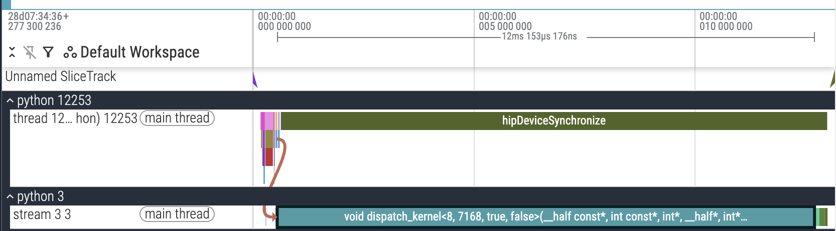
PyTorch Profiling trace, showing unusually slow dispatch-send.
I narrowed down the issue to the spin-lock loop of the token count. My best guess is that the AMD profiler backend has strange interactions with multi-GPU code. Anyway, due to this issue, I switched to manual CUDA events timing (submission_v6.py#L893-L913), and obtained the following results for the largest problem shape (num_experts=256, experts_per_token=8, hidden_dim=7168, max_num_tokens=256, world_size=8).
| Rank | Dispatch | Grouped GEMM | Combine | Total |
|---|---|---|---|---|
| 0 | 348.60 | 115.66 | 342.94 | 807.20 |
| 1 | 334.80 | 115.98 | 342.18 | 792.97 |
| 2 | 377.98 | 115.78 | 333.76 | 827.53 |
| 3 | 330.19 | 115.30 | 317.28 | 762.78 |
| 4 | 333.96 | 115.22 | 349.44 | 798.62 |
| 5 | 314.84 | 115.46 | 326.59 | 756.89 |
| 6 | 327.07 | 115.02 | 325.34 | 767.43 |
| 7 | 329.03 | 115.42 | 336.49 | 780.94 |
So far, I focused only on dispatch and combine, leaving “faked” grouped GEMM alone. Profiling data showed that grouped GEMM contributes quite a bit to the overall runtime. Fusing it with combine would reduce latency by ~100μs, and it was simple too: “fake” grouped GEMM was just a pointwise multiplication. After checking with the organizer that it was a valid optimization, I implemented it and reduced the runtime to 421μs.
- For an actual MoE kernel, we can still do fusion:
combinecan be fused with grouped GEMM’s epilogue. However, there are new complications as well: slow epilogue leaves SM/CU’s compute units idle without additional tricks like warp specialization; GEMM tile-based output is not directly compatible with per-token lock design.
Kernel tuning
Generally, I don’t want kernel tuning to have its own section, since technically all kernels should be re-tuned when there is a change, regardless of how small it is. However, sometimes tuning reveals certain properties of the device that are worth discussing.
For my kernels, I can tune grid_size (number of threadblocks) and NUM_WARPS (number of warps in a threadblock). All of my code written so far is agnostic to these hyperparameters, so tuning them is easy. Setting grid_size=304 (exactly the number of CUs in MI300X) for combine resulted in end-to-end latency of 345μs! This was quite surprising, as the number of threadblocks must exactly be 304. Any other reasonably large number like 256 would not achieve the same speedup.
Using grid_size=256 for combine.
| Rank | dispatch-send | dispatch-recv | combine-send | combine-recv | Total |
|---|---|---|---|---|---|
| 0 | 225.99 | 78.78 | 300.92 | 46.26 | 651.96 |
| 1 | 225.35 | 77.50 | 310.66 | 53.48 | 666.99 |
| 2 | 289.38 | 38.29 | 311.23 | 47.15 | 686.03 |
| 3 | 289.58 | 32.51 | 299.80 | 49.71 | 671.60 |
| 4 | 231.08 | 77.17 | 307.38 | 62.30 | 677.94 |
| 5 | 211.76 | 90.44 | 302.80 | 65.03 | 670.04 |
| 6 | 279.92 | 32.95 | 292.10 | 48.07 | 653.04 |
| 7 | 205.35 | 87.68 | 305.97 | 47.99 | 646.99 |
Using grid_size=304 for combine.
| Rank | dispatch-send | dispatch-recv | combine-send | combine-recv | Total |
|---|---|---|---|---|---|
| 0 | 219.33 | 95.70 | 108.88 | 60.02 | 483.93 |
| 1 | 216.93 | 106.40 | 115.42 | 50.75 | 489.50 |
| 2 | 283.88 | 64.19 | 117.95 | 46.54 | 512.56 |
| 3 | 291.94 | 32.27 | 97.66 | 56.09 | 477.96 |
| 4 | 236.97 | 60.94 | 126.17 | 43.06 | 467.13 |
| 5 | 211.08 | 106.96 | 113.14 | 54.24 | 485.41 |
| 6 | 304.65 | 32.83 | 113.46 | 46.02 | 496.96 |
| 7 | 214.08 | 106.68 | 113.17 | 52.04 | 485.97 |
grid_size=304 gives a near 3x speedup for combine-send! Like with many other observations on MI300X, I had no explanations. Tuning dispatch didn’t yield any noticeable speedup.
Eliminate overheads
I mentioned that PyTorch Profiler didn’t show very meaningful traces in the previous section, but occasionally it was fine on some ranks. Inspecting one of such traces revealed unacceptable overheads coming from dynamic allocations (malloc) and zeroing out buffers (memset).
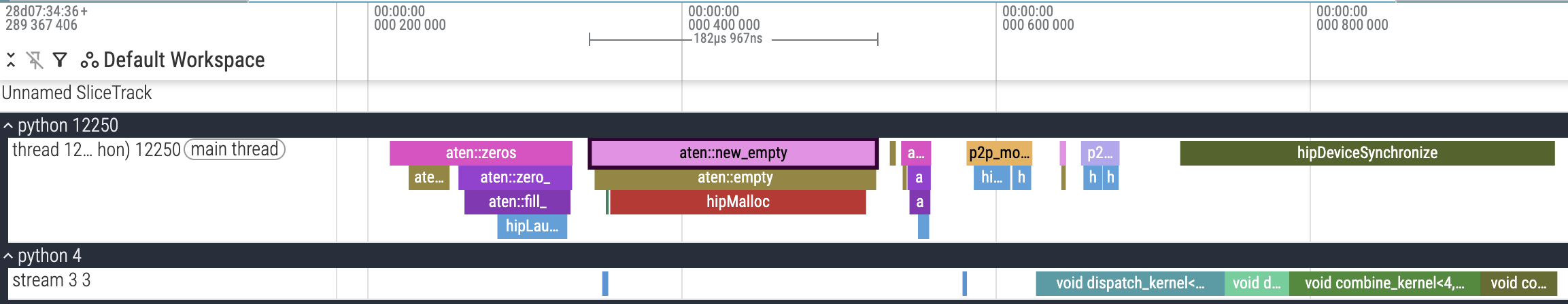
Malloc and zeros overheads.
It was strange that there were hipMalloc calls, as PyTorch’s caching allocator should have taken care of them. Regardless, eliminating malloc calls was simple - move torch.empty() outside of the main kernel, and reuse the buffers.
Zeroing out buffers was more problematic. In my kernels, I rely on the fact that the buffers are initialized with zeros for correct logic, such as token count with atomicAdd(). One solution is to switch to cudaMemsetAsync() in C++ to remove Python overheads as well as unnecessary kernel launches, but I think we can do better.
The main idea is that we can sneak in memset in later kernels to restore the invariance. Logically, we are doing the following.
# allocation, initialized to zeros
send_counts = torch.zeros(WORLD_SIZE)

# call the kernel multiple times
for _ in range(10):
    dispatch_send(..., send_counts)
    send_counts.zero_()  # restore invariance
    dispatch_recv(...)
    ...
To avoid a separate kernel (or cudaMemsetAsync()) for send_counts.zero_(), we can fuse it with the next kernel dispatch-recv. Since this buffer is small, using some threads in the 1st threadblock is enough.
// STAGE: dispatch-recv
// reset send_counts buffer used in dispatch-send
// since zero_() is very expensive
if (bid == 0 && tid < WORLD_SIZE)
  send_counts[tid] = 0;
As I was already doing overhead reduction, I also moved most of the code to C++, including slicing of the symmetric heap. Hence, submission_v7b.py focused solely on removing overheads, achieving 303μs.
Optimize varlen work distribution
Intra-kernel profiling
One of the coolest tricks that I learned from my teammate was intra-kernel profiling. CUDA events (and PyTorch Profiler) can only do profiling at the kernel level - how long a particular kernel, or a group of kernels, takes. To understand the bottleneck at the code level, we need to profile within the kernel itself.
For NVIDIA GPUs, usually I will use Nsight Compute’s Source view to check which line of code accounts for the most warp stalls. I couldn’t find the equivalent for AMD, hence the intra-kernel profiling trick was particularly useful.
The goal is to produce a Chrome trace that I can visualize with https://ui.perfetto.dev/. The format is quite simple - we only need the starting and ending timestamps of a particular event, and some extra metadata. To obtain a timestamp within a kernel on AMD GPUs, I borrowed the code from Iris.
__device__
int64_t read_realtime() {
  int64_t t;
  asm volatile("s_waitcnt vmcnt(0)\n"
               "s_memrealtime %0\n"
               "s_waitcnt lgkmcnt(0)" : "=s"(t));
  return t;
}
Once we have the timestamps, we can write them to global memory. The tricky thing is to annotate events of different types, which may come from multiple threads or threadblocks at the same time. I came up with a simple scheme.
__device__
int profile_start(int64_t *profile) {
  int i = atomicAdd(reinterpret_cast<int*>(profile), 1);
  profile[1 + i * 4] = read_realtime();
  return i;
}

__device__
void profile_stop(int64_t *profile, int i, int tag, int tid) {
  profile[1 + i * 4 + 1] = read_realtime() - profile[1 + i * 4];
  profile[1 + i * 4 + 2] = tag;
  profile[1 + i * 4 + 3] = tid;
}

// usage
{
  // obtain event ID
  int e0_id;
  if constexpr (DO_PROFILE) if (tid == 0) e0_id = profile_start(p2p_state.profile);

  // code being recorded
  ...

  // use the previous event ID to write down ending timestamp
  if constexpr (DO_PROFILE) if (tid == 0) profile_stop(p2p_state.profile, e0_id, 0, bid);
}
int64_t *profile is just a buffer in global memory. Its first element profile[0] is the number of events recorded so far, thus atomicAdd() returns the index of a new event to be recorded. After the first element, each event occupies 4 elements:
- Starting timestamp
- Ending timestamp
- Numerical tag
- ID
This design allows multiple threads to record their events independently without ahead-of-time layout planning. The numerical tag can be looked up later with a list of names. To add new event names, we can add more elements to this lookup list.
Uneven work distribution
With the ability to do intra-kernel profiling, we can now obtain a more fine-grained trace of the kernel. I recorded the sending and receiving events of each token, for both dispatch and combine. I also merged the traces of all GPUs into a single file for ease of visualization.
- Chrome’s
pid(Process ID) is mapped to GPU rank, Chrome’stid(Thread ID) is mapped to GPU threadblock ID. For each threadblock, I only recorded the first warp. - There are some quirks in Chrome trace format and/or UI Perfetto. For
pid=N,tidmust start withN. To display the data correctly, I had to increment threadblock IDs for rank N byN. Thus, in the screenshot below, for Process 4, you should subtract Thread ID by 4 to obtain the original threadblock ID.
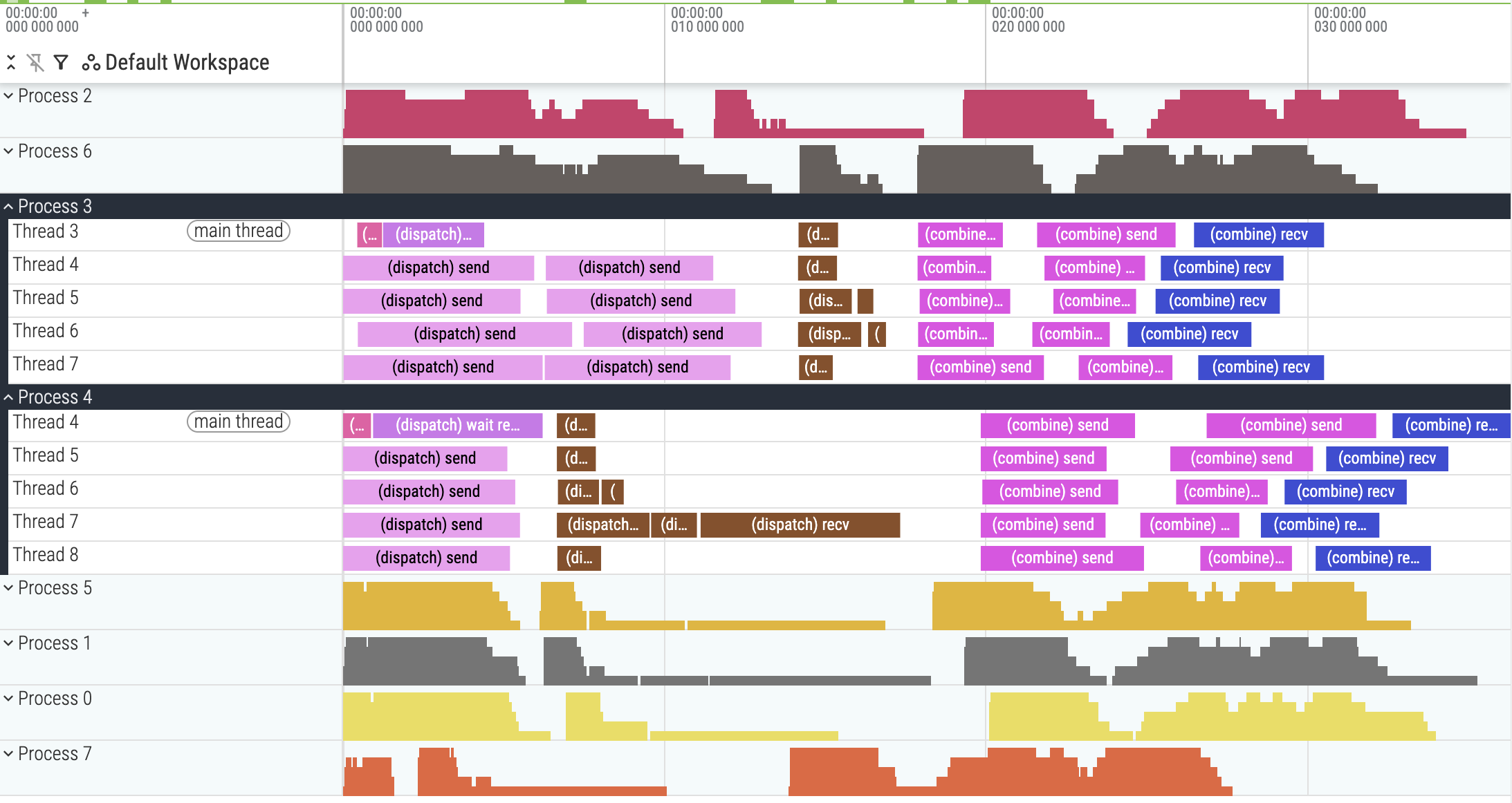
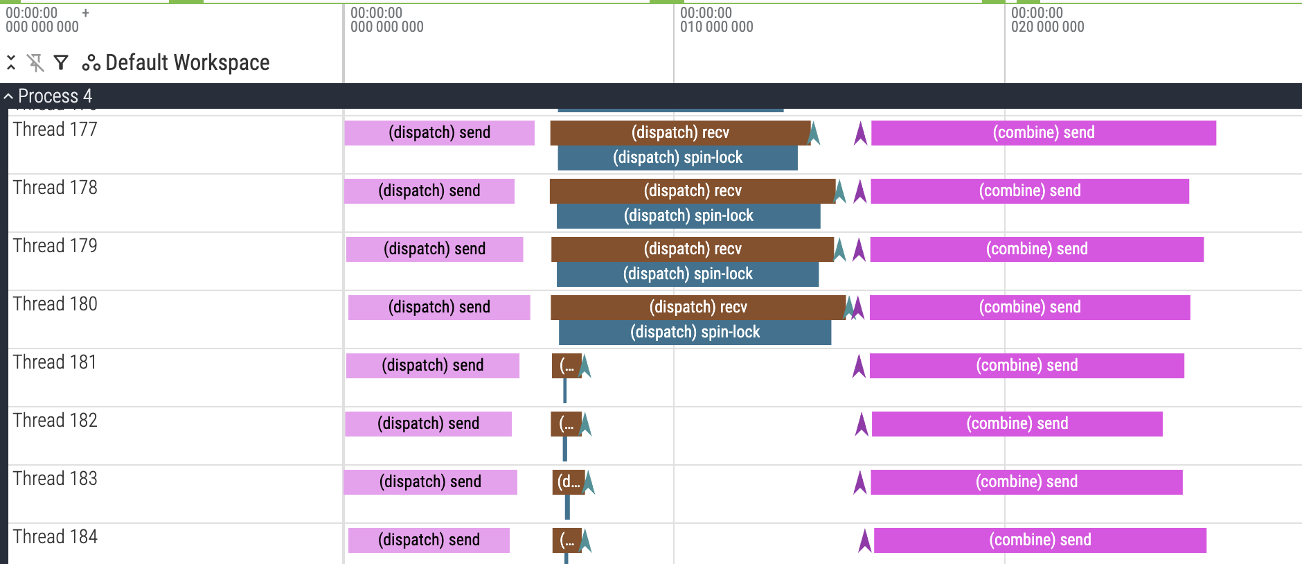
trace_v8.json.gz. Intra-kernel profiling of v8, showing uneven work distribution across threadblocks in dispatch-recv. Process 4 Thread 4 means GPU4 threadblock 0.
There was an obvious uneven work distribution in the dispatch-recv kernel. Process 4 Thread 7, which mapped to GPU4 threadblock 3, had to receive 3 tokens, while most other threadblocks only received 1 token. This was due to the way I distributed work among threadblocks in dispatch-recv.
// each block is assigned a src_rank based on its bid (round-robin)
// hence, each src_rank is handled by (num_blocks / WORLD_SIZE) threadblocks
const int src_rank = bid % WORLD_SIZE;
const int recv_count = comm_recv_counts[src_rank];

// each warp handles 1 token
// divide by WORLD_SIZE due to src_rank assignment above
for (int comm_pos = (bid / WORLD_SIZE) * NUM_WARPS + warp_id;
  comm_pos < recv_count;
  comm_pos += (num_blocks / WORLD_SIZE) * NUM_WARPS) {
  // spin-lock and token copy
  ...
}
If there are more tokens coming from a particular rank, threadblocks assigned to that rank need to do more work than the rest. In the profiling trace above, GPU4 threadblock 3 (Process 4 Thread 7) was receiving tokens from GPU3, which was sending more tokens than other ranks were. Ultimately, this is a problem of work distribution when there are variable-length sequences.
I know that the varlen version of Flash Attention additionally takes in sequence offsets (i.e. cumulative lengths) and max sequence length. This is similar to the varlen torch._grouped_mm() introduced previously. I can kinda guess the threadblock partitioning logic without inspecting the source code, but there is a problem: we need the cumulative sum of token counts coming from other ranks, which then requires a grid-wide synchronization.
Or do we? There are only 8 items, so it doesn’t cost much for all threads to do the cumulative sum independently.
// RECV stage
// "flatten" the recv tokens from all other ranks -> ensure work is distributed across all threadblocks equally,
// even if recv tokens from other ranks are not even.
int idx = bid * NUM_WARPS + warp_id;
int start = 0; // start of current src_rank
for (int src_rank = 0; src_rank < WORLD_SIZE; src_rank++) {
  int end = start + comm_recv_counts[src_rank]; // end of current src_rank

  for (; idx < end; idx += num_blocks * NUM_WARPS) {
    // spin-lock and copy token
    ...
  }

  start = end;
}
Conceptually, the above is equivalent to
for (int idx = bid * NUM_WARPS + warp_id;
  idx < sum(comm_recv_counts);
  idx += num_blocks * NUM_WARPS) {
  ...
}
which distributes work across threadblocks evenly. There are some overheads, as the inner loop might be empty, but I think it’s pretty minimal for this problem.
I also applied the same logic for combine-send, as it also handled varlen sequences coming from num_local_experts sequences. This became submission_v9.py, which was my final version. End-to-end runtime did not improve much, only reached 292μs.
Uneven work stalling
Despite our improved work distribution, dispatch-recv didn’t get much faster.
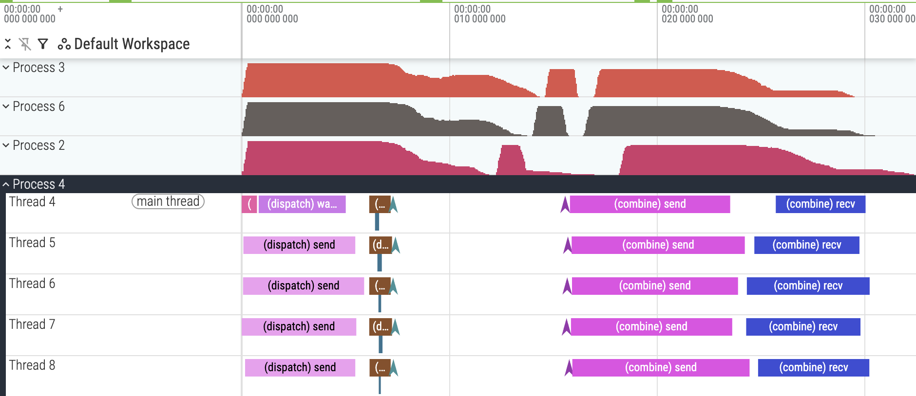
trace_v9.json.gz. Intra-kernel profiling of v9, showing dispatch-recv stall.
I was perplexed at the white gap between dispatch-recv and combine-send at first (why didn’t combine-send start earlier?), but inspecting later threadblocks revealed the answer.
trace_v9.json.gz. Intra-kernel profiling of v9, showing uneven dispatch-recv’s spin-lock time across threadblocks.
Due to our new threadblock work distribution, it was not obvious which source rank a threadblock was handling. The sharp difference between Thread 180 and Thread 181 in the Chrome trace above probably corresponds to an increment in source rank.
- We could verify this by adding extra annotations to our profile events, but I didn’t implement it.
Zooming out the Chrome trace, you can see some ranks send more data than the others. Hence, threadblocks with unusually slow spin-lock loops were actually waiting for data from those ranks to arrive.
- I highly recommend that you download the Chrome trace from the link above to visualize and interact with it by yourself, since I can’t show everything through screenshots.
- In this competition, the number of tokens from each rank is not the same, which I think is pretty unusual for a typical DP deployment (due to load balancing).
Though I could identify the problem, I ran out of time to implement any useful improvements. I believed a pipelining approach like in Comet could help: by splitting the data into 2 (or more) partitions, we can run the full series of kernels on a subset without waiting for all tokens to finish execution.
Closing remarks
Here is a summary of my progressive improvements across versions.
| Version | Code | Leaderboard runtime |
|---|---|---|
| Reference | reference.py | 93540μs |
| Optimized PyTorch-only | submission_v2.py | 1311μs |
| P2P symmetric memory | submission_v5.py | 517μs |
| Fuse grouped GEMM + combine. Tuned kernel | submission_v7.py | 345μs |
| Remove overheads | submission_v7b.py | 303μs |
| Varlen work distribution | submission_v9.py | 292μs |
The iteration process was definitely not monotonic: ideas didn’t pan out, some implementations were slower than their previous versions. But I hope this worklog reveals a logical process when tackling a new kernel.
It was unfortunate that I didn’t have time to tinker with the other two problems in the competition: gemm-rs and ag-gemm. My teammate released his solutions at benenzhu/gpu-mode-kernels. You definitely should check them out!
Lastly, I would like to thank the following people, without whom this blog post wouldn’t be possible:
- The competition organizers, AMD and GPU MODE, for giving me the opportunity to learn about multi-GPU programming.
- zhubenzhu, my accidental teammate, with whom I exchanged numerous cool ideas and knowledge. Per-token flag design and the intra-kernel profiling trick were from him.
- Iris’s authors for creating such an elegant library. Their GPU MODE lecture was my first introduction to multi-GPU programming. Even though I didn’t use Iris directly, it was instrumental to my understanding of symmetric memory and various tricks for AMD GPUs.
- Yotta Labs for sponsoring the compute for our kernel development.